
There is a function in Excel called CELL. It returns information about a cell, but it has some very strange characteristics and quirks.
The inputs appear straight forward. =CELL(info_type, [reference])
The info_type will show up as a choice of words, some seem obvious as to what they will return, others are a bit more obscure.
As usual, the input in square brackets is optional, but in this case it is highly recommended, as without it the behaviour of the function will appear erratic unless you fully understand what it is doing.
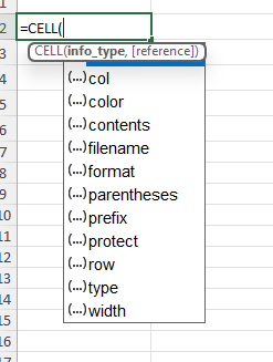
You can see the list of options for the first input. Select the one you require.
For the second input, put the cell reference to the cell you want to know about. If you don’t put anything (it is optional after all) then the formula will return information about the cell that is “selected at the time”. So, if you click somewhere in the spreadsheet, you will get information about the selected cell when the spreadsheet recalculates. And this behaviour is different on different platforms, it all gets a bit complex. For a full explanation of all the ins and outs see the Microsoft website.
Note too, that CELL is a volatile function, which means it can slow your spreadsheet down if it is large or very complex.
Even some of the inputs are not quite as they appear. Color for example, does not actually bring back the colour of the reference. It is actually referring to whether or not the reference is formatted to show negative values in a different colour. Likewise, format, paratheses, and prefix are all to do with how the cell is formatted. The others are as they appear but see the link above to get the detail.